SAXS Fingerprint Atlas
GALLERY
This atlas is an introductory guide for those new to Small-Angle X-ray Scattering (SAXS) or looking to learn the basics of data interpretation. It reproduces typical SAXS patterns using simulations; by observing the characteristic 'fingerprints' of each pattern and using simple formulas (calculable even with a basic calculator), you can derive approximate structural information with ease.
To extract more detailed information, it is effective to perform model-based fitting calculations or to compare with Small-Angle X-ray Scattering pattern simulations based on molecular dynamics simulation results.
*Note: In actual data analysis, these patterns should be compared after appropriately subtracting background scattering from solvents or other sources.
 No. 01
Spherical Particles
 No. 02
Aggregated Spheres
 No. 03
Concentrated Spheres
 No. 04
Core-Shell Spheres
 No. 05
Rods & Disks
 No. 06
Lamellar Structure
of Rods
 No. 07
Gaussian Chain
(Random Coil)
 No. 08
Random
Network
 No. 09
Disordered
Bicontinuous
 No. 10
Ordered
Bicontinuous
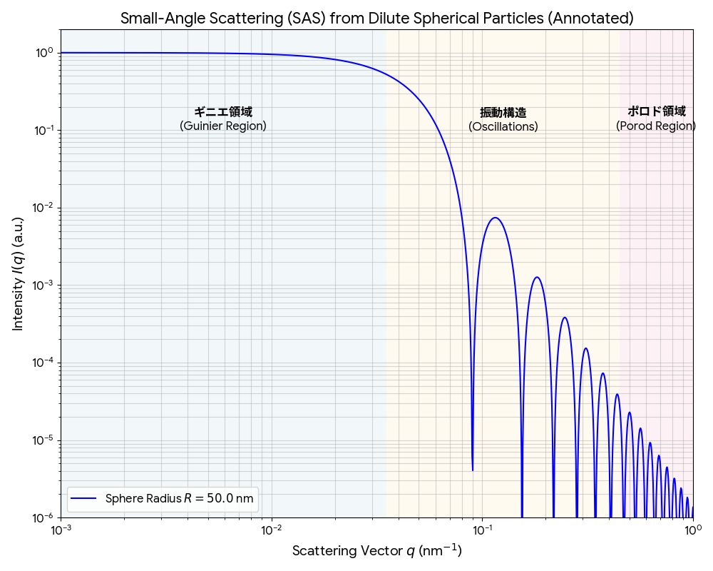
No. 01 [Basic Form] Dilute Spheres
The scattering pattern of a dilute dispersion of spherical particles is the starting point of all analysis. A ruler to understand what profile 'uniform, non-interfering particles' describe.
1. 'Fingerprint' to look for on site
- Low angle (left side): A flat 'plateau' where the intensity becomes constant.
- Mid-to-high angle: A series of regular 'dips' and 'peaks'.
2. Main Analytical Indicators
- Size evaluation by Guinier Plot: From the initial slope a when plotted with q2 on the x-axis and ln I(q) on the y-axis, the particle size (radius of gyration Rg) is calculated as:
Rg = √(−3×a) - Estimation from the dip position: From the position of the first dip qmin1, the physical radius R can be calculated:
R ≈ 4.49 / qmin1
Thus, the approximate particle size can be cross-checked using both the Guinier plot and the dip position. - High-angle Decay (Porod's Law): Focus on the decay slope in the high-angle region (Porod region) on the right side of the graph. For spherical particles with smooth interfaces, the intensity decays proportional to q−4. This reflects the 'surface smoothness' of the particle; deviations occur if the interface is rough.
3. Effect of Particle Size Distribution (Polydispersity) on Profiles
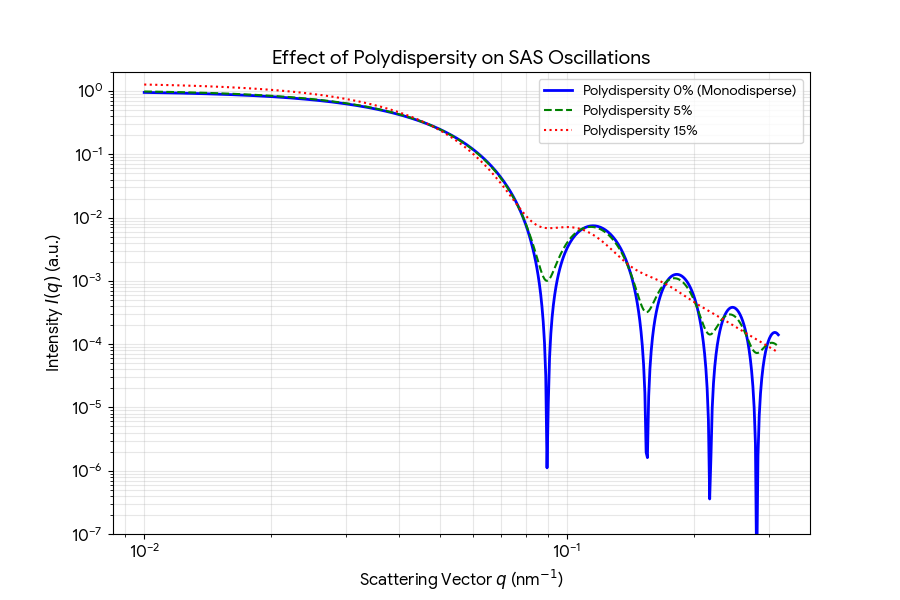
This graph illustrates three cases with different levels of particle radius variation (polydispersity: σ).
- Blue Solid Line (0% / Monodisperse): An ideal state where all particles are identical in size. The dips are extremely deep and sharp, showing the clearest profile features.
- Green Dashed Line (5%): A state with a narrow size distribution. While the ideal shape is maintained, the sharp dips become shallower and features start to blur.
- Red Dotted Line (15%): A state with a broad size distribution. The deep dips disappear completely, resulting in a smooth decay curve.
Main Analytical Indicators
- 'Dip Depth' as an Indicator of Uniformity: If sharp dips are observed in the measured data, it is definitive proof that the nanoparticles are extremely uniform in size.
- Interpreting Smooth Decay Curves: Even if the dips are absent and the profile appears as a smooth slope (red line), it serves as crucial evidence of the presence of particles with a wide size distribution.
- Quick Assessment of Distribution: By comparing the number and depth of visible dips with this graph, one can estimate the approximate size distribution on-site without complex fitting analysis.
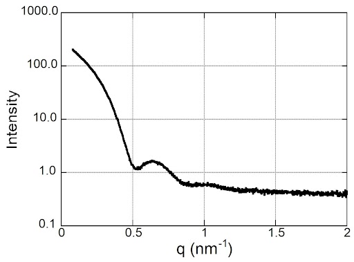
Analysis of Actual Measurement Data: Gold Nanoparticles using BL08W SAXS
Exposure time: 60 sec
X-ray energy: 8.0 keV
1. Particle size is approximately 20 nm in diameter
In the graph, the scattering intensity shows the first dip near q ≈ 0.5 nm−1. In SAXS of spherical particles, the first minimum of the form factor appears around qR ≈ 4.49. Therefore, R ≈ 4.49 / 0.5 ≈ 9 nm, which means the diameter is estimated to be about 18 nm. This matches well with the "average particle size of approx. 20 nm".
2. Particles are nearly spherical
The dip near q ≈ 0.5 nm−1 and the subsequent weak oscillations (hills/shoulders) are typical features of the form factor of spherical nanoparticles. If the sample consisted only of rods, plates, or irregular aggregates, such characteristic spherical oscillations would be less likely to appear.
3. Size distribution exists but doesn't seem extremely broad
While oscillations are visible, the peaks and dips are quite rounded and not sharp. This suggests that the particle size is not perfectly uniform but has a certain degree of size distribution. This is a natural appearance for a gold nanoparticle dispersion with an average particle size around 20 nm.
4. No prominent regular arrangement or strong aggregation is observed
Since no sharp peaks are seen across the entire q range, a structure where particles are arranged crystallographically or periodically is not strongly indicated. Although the intensity is high at low q, it is difficult to confirm clear structural peaks indicating strong aggregates or long-range order from the published figure alone.
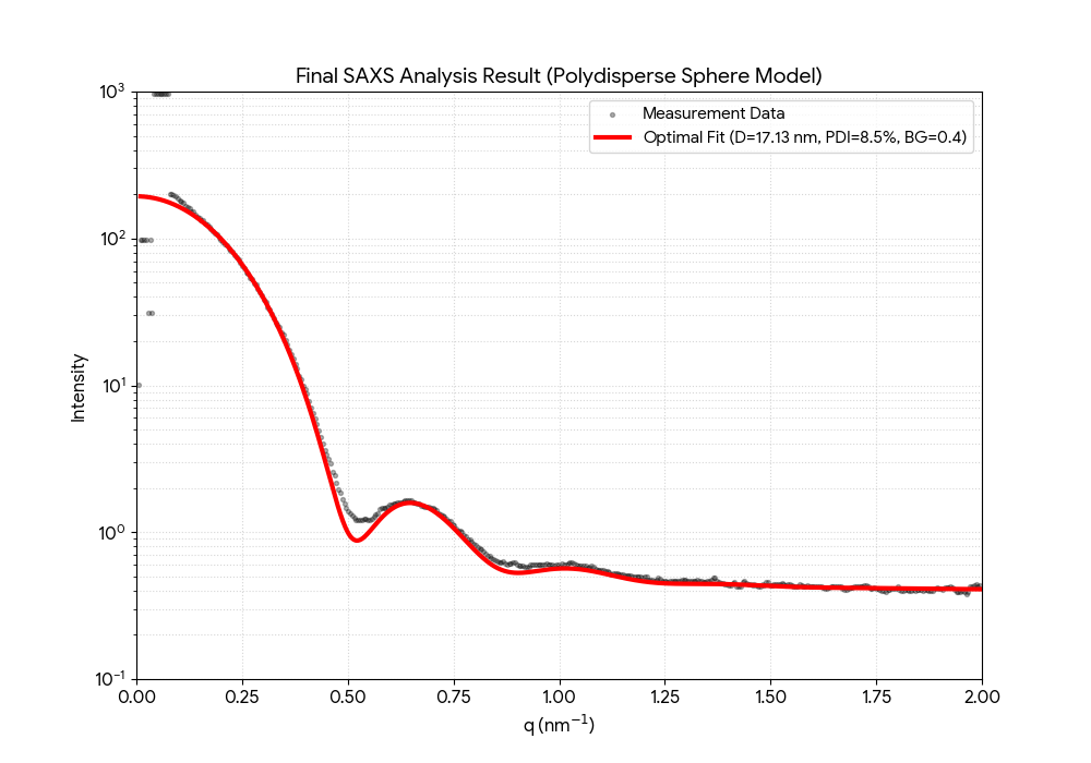
- - Avg. Particle Size (Diameter D): 17.13 nm
- - Polydispersity (σ/R): 8.5%
- - Background Intensity (BG): 0.40
*Result of least-squares fitting using a polydisperse sphere model (Schulz-Zimm distribution).
(Fitting program created and executed by Google Gemini)
*It is highly likely that the actual gold core itself is approximately 17 nm, and it is marketed as "20 nm" (nominal size or DLS measurement) as a total particle size including the surface layer.
1. Surface State (Porod's Law)
The intensity decay around q ≈ 0.8–1.2 nm−1 follows q−4 (Porod's Law), indicating a very sharp interface between the particles and the solvent, as well as a smooth particle surface. Rough surfaces or fuzzy boundaries would result in a more gradual slope.
2. Uniformity of Internal Structure
The profile is exceptionally well-described by a uniform sphere model, suggesting a homogeneous internal structure with constant electron density. Core-shell or hollow structures would produce more complex scattering patterns.
3. Interpretation of the Low-Angle "Upturn"
The slight intensity rise around q ≈ 0.1 nm−1 suggests the presence of minor fine aggregates (such as dimers) or background scattering from structures much larger than the particles themselves (e.g., bubbles or dust in the liquid).
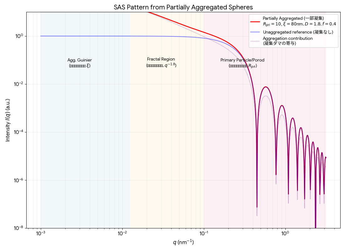
No. 02 Aggregated Spheres
A state where particles are not isolated but stick together to form 'aggregates'.
1. Common points with No. 01
- High-angle behavior: If the 'original particle shape' is maintained even when aggregated, dips and peaks appear at the same positions as No. 01. You can confirm the primary particle size here.
Characteristic Differences
- Upturn at low angles: The flat low-angle region in No. 01 changes to a steep upward slope.
- Fractal slope: The slope (−D) connecting the aggregate plateau and the primary particle shoulder indicates whether the inside of the aggregate is 'sparse' or 'dense'.
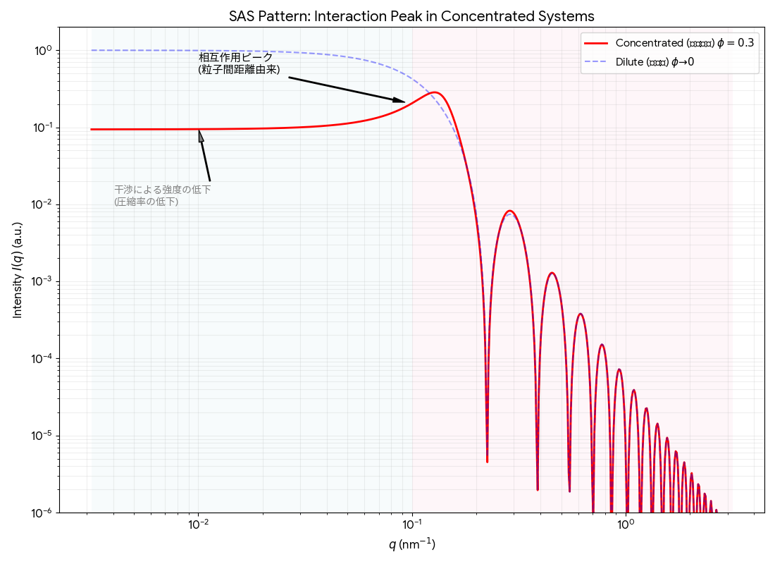
No. 03 Concentrated Systems
A state where particles are densely packed and their arrangement is restricted by excluded volume.
1. Common points with No. 01
- High-angle convergence: Above q > 0.2, the shape of the particles themselves does not change, perfectly matching the form factor P(q) of No. 01.
Characteristic Differences
- Interaction Peak: A distinct peak appears where there was only a 'shoulder' in No. 01. Using this peak position qpeak, the average distance between particles can be calculated:
d (interparticle distance) ≈ 2π / qpeak - Low-angle intensity suppression: Due to interparticle interference (repulsive correlation), the intensity at the left edge becomes lower than No. 01 (dilute system).
NanoTerasu Application Advice
With NanoTerasu, the data needed for pattern identification can be obtained in just a few seconds. First, take a measurement and apply the No. 01 'ruler'. If the left end is upturned, it's No. 02 (aggregation); if a peak is visible, it's No. 03 (concentrated).
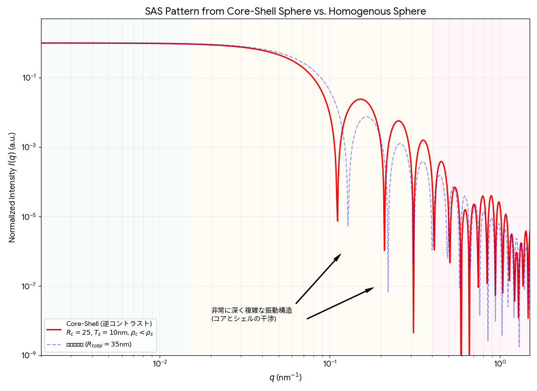
No. 04 Core-Shell Type Particle (Double Spherical Structure)
A dual-structure pattern with different densities inside and outside, such as 'particles coated with polymer'.
1. Common points with No. 01
- Low-angle plateau: Flat shoulder similar to No. 01, reflecting the radius of gyration Rg of the 'core + shell total size'.
- High-angle Porod slope: Converges to a slope of −4, just like No. 01.
Characteristic Differences (The 'Fingerprint'!)
- Complex and deep oscillatory structure: Compared to a simple sphere (No. 01), core-shell particles show very deep and complex periodic dips. This is due to interference between scattering waves from the core and the shell.
3. Main Analytical Indicators
- Checking deviation from 'homogeneous sphere': If the dip positions are shifted or certain peaks are enhanced compared to a homogeneous sphere of the same outer diameter, it is definitive proof of a 'core' with a different density.
- Contrast reversal: If the shell density differs significantly from the solvent or core, the amplitude of these oscillations becomes even more intense. This 'complexity of waving' holds the key to information about the shell thickness and density.
NanoTerasu Application Advice
In the analysis of core-shell structures, the 'density difference (contrast)' between the core and shell is crucial. Using NanoTerasu's high-brightness beam, even when the shell is extremely thin or the density difference is slight, these 'deep dips due to interference' can be captured vividly. Before counting hundreds of particles with an electron microscope to confirm if coating was successful, measure for a few seconds with SAXS and overlay the profile with No. 01 (homogeneous sphere) from this atlas. If the positions and depths of the dips do not match, it is a sign of successful coating.
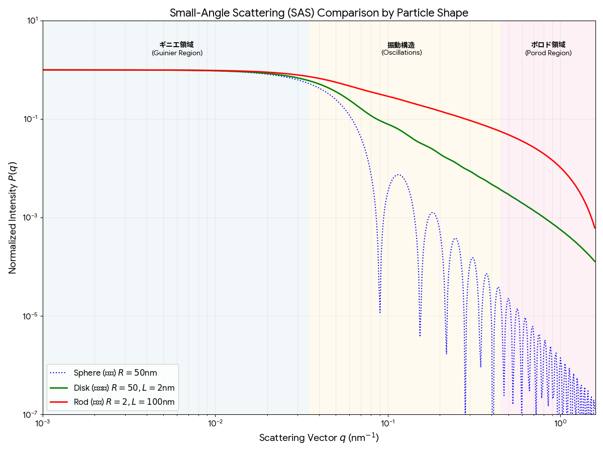
No. 05 Rods & Disks
A state where the 'spherical ruler' is stretched or compressed. As the shape changes from a 'sphere' to a 'rod' or 'disk', the decay rate and curvature of the scattering change dramatically.
1. 'Fingerprint' to look for (log-log plot)
- Rod (red line): Decays with a slope of −1.
- Disk (green line): Decays with a slope of −2.
2. Main Analytical Indicators (Cross-section/Thickness)
After identifying the shape, by switching to a dedicated plot axis, 'thickness' and 'cross-section' can be calculated without complex analysis.
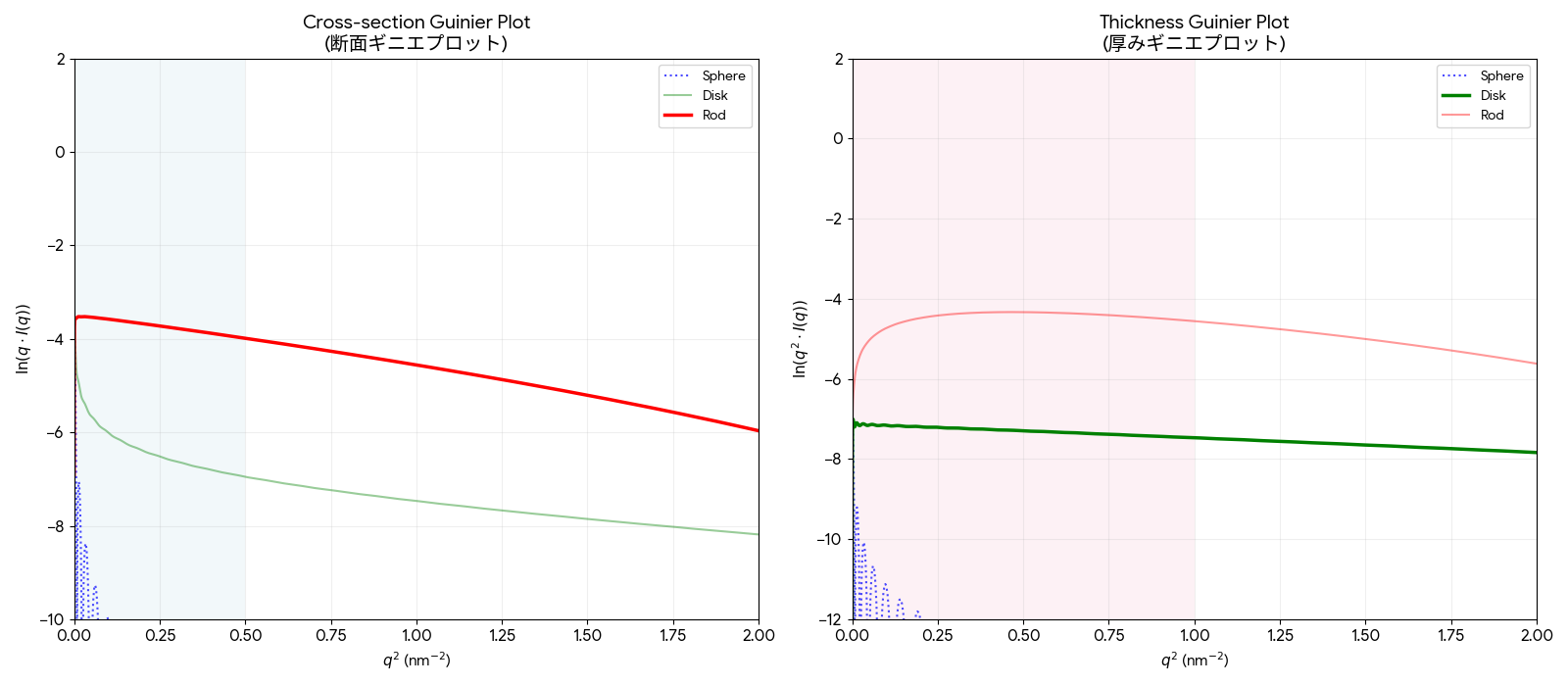
- A. Rod 'Thickness' (Cross-sectional Guinier): Plot ln(q · I) vs q2. The cross-sectional radius of gyration Rgc is calculated from the slope a:
Rgc = √(−2a) - B. Disk 'Thickness' (Thickness Guinier): Plot ln(q2 · I) vs q2. The thickness radius of gyration Rgt is calculated from the slope a:
Rgt = √(−a)
3. Analysis Hint: Confirming Dimensionality
- q−1 slope + linear cross-sectional Guinier plot = Clean rod/line shape
- q−2 slope + linear thickness Guinier plot = Clean disk/sheet shape
4. How to Distinguish from Flexible Polymers and Networks
- Disk vs. Gaussian Chain (No. 07): Both show a −2 slope in the intermediate region. However, disk-shaped particles show a sharp intensity drop off at high angles due to their 'thickness' (form factor), whereas Gaussian chains maintain scattering intensity without such a drop.
- vs. Random Network (No. 08): Rods and disks have clear intermediate slopes (−1 or −2) indicating their dimensionality. In contrast, random networks like the Debye-Bueche type decay smoothly from a plateau directly to a −4 slope without showing specific dimensionality.
NanoTerasu Application Advice
Even if rod-like or disk-like particles are in 'random orientation' without a specific direction in solution, SAXS can clearly distinguish their geometric 'dimension'. Before capturing a single particle in detail with ptychography, first use SAXS to obtain supporting evidence for whether the sample as a whole is a 1D rod or a 2D sheet.
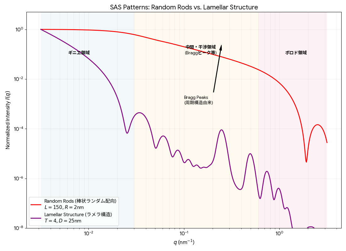
No. 06 Lamellar Structure formed by rods
A 'stacked membrane' structure seen in surfactants, lipid membranes, or lamellar polymers.
1. 'Fingerprint' to look for
- Periodic sharp peaks (Bragg Peaks): Equally spaced sharp peaks appear. This is definitive evidence of 'stacked layers'.
- Overall decay (envelope): The overall shape connecting the peaks decays along a slope of −2, reflecting its 2D nature.
2. Main Analytical Indicators
The main parameters of the lamellar structure, the period D and the membrane thickness T, can be calculated. (D−T=W represents the gap between membranes)
- A. Period D: Let the first peak position be qpeak1:
D (period) ≈ 2π / qpeak1 - B. Membrane thickness T: Focus on the position where the intensity drops sharply and then rises again (due to the form factor effect). (In the above graph, around q = 1.57 nm−1)
T ≈ 2π / qmin_envelope
NanoTerasu Application Advice
Lamellar structures change dramatically with temperature, concentration, and solvent conditions. With NanoTerasu's high-brightness, high-speed measurement, changes in peak positions (period D) and envelope shape (thickness T) can be tracked in real-time.
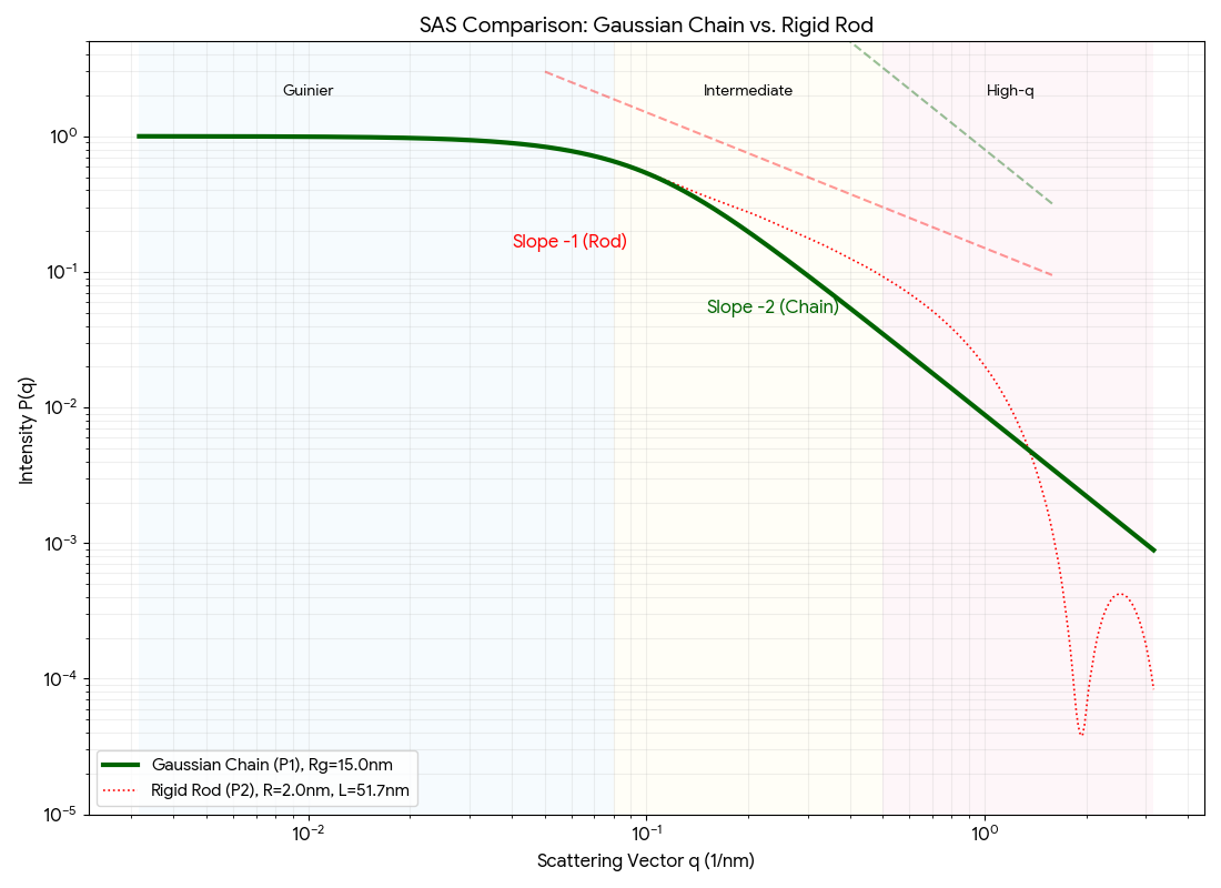
No. 07 Gaussian Chain / Polymer
Pattern of a polymer freely wiggling in solution (random coil). Shows a very different fingerprint from 'hard particles'.
1. 'Fingerprint' to look for
- No oscillations: Smooth curve over the entire region without any dips or peaks, because the density distribution is spatially 'blurred'.
- Mid-region slope −2: Gaussian chains decay with a slope of −2 (statistical 2D nature), compared to −1 for rods.
2. Main Analytical Indicators
- Check if slope is −2: If intensity drops proportional to q−2 in the intermediate region, it is evidence of a 'flexible chain' rather than a 'hard rod'.
3. How to Distinguish from Other Structures (Rods, Disks, Random Networks)
- vs. Rods (No. 05) - Dimensionality: Rods decay with a slope of −1 (1D), whereas Gaussian chains decay with a slope of −2 (statistical 2D). Even with the same radius of gyration (Rg), this slope helps determine whether it's a 'rigid' or 'flexible' structure.
- vs. Disks (No. 05) - Presence of Interfaces: Both show a −2 slope, but disks exhibit a sharp drop at high angles due to their 'thickness' (form factor). Gaussian chains maintain scattering at high angles.
- vs. Random Networks (No. 08) - Sharpness of Interfaces: Gaussian chains decay slowly at −2, but Debye-Bueche types decay rapidly at −4 because they have distinct density boundaries (interfaces).
NanoTerasu Application Advice
In the analysis of polymer materials, this 'slope -2' is the basis. If the slope is -5/3 (≈ 1.67), it indicates that the solvent affinity is very high and the molecular chain is swollen.
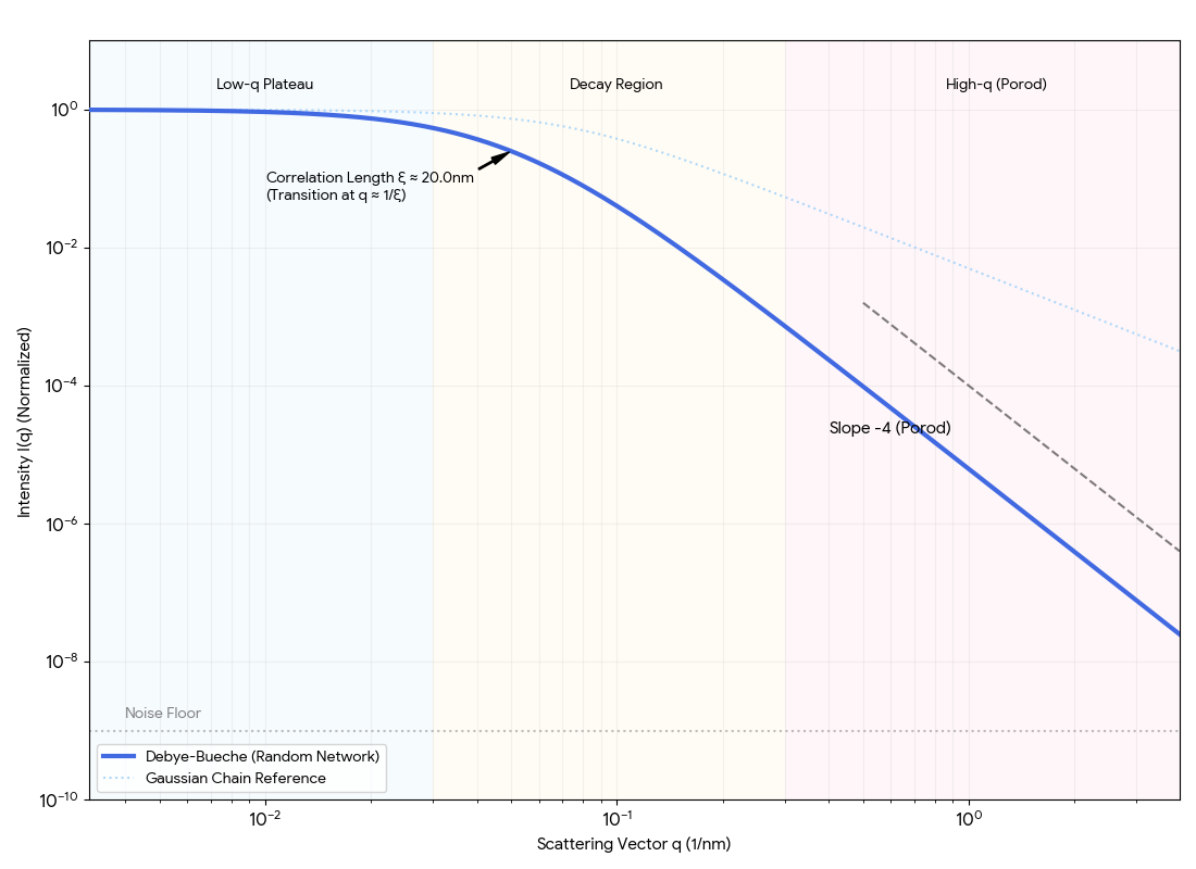
No. 08 Random Network (Debye-Bueche Type)
The fingerprint of a system without specific shapes (spheres or rods), where density fluctuations are spatially distributed at random. Frequently seen in porous materials, polymer gels, or inhomogeneous alloy structures.
1. 'Fingerprint' to look for
- No Characteristic Structural Peaks: Focus on the thick blue solid line. The 'humps' seen in Bicontinuous structures (No. 09, No. 10) do not appear at all.
- Gentle Decay: Intensity drops consistently from a flat plateau on the low-angle side towards the high-angle side.
- High-angle Porod Decay (−4): As q increases, it perfectly matches the q−4 slope (gray dashed line), indicating the presence of a distinct interface.
2. Main Analytical Indicators
Identify the average size of the random density fluctuations (correlation length ξ).
- Debye-Bueche Plot: Plot with q2 on the x-axis and 1/√I(q) on the y-axis.
1/√I(q) = (1/√I(0)) × (1 + ξ2q2)
The correlation length ξ is determined from the slope of the line.
Rule of thumb: ξ ≈ 1 / qtrans, where qtrans is the position where the graph starts to bend.
3. How to Distinguish from Gaussian Chains and Shaped Particles
- vs. Gaussian Chain (No. 07) - Presence of Interfaces: Gaussian chains decay slowly at q−2 without 'clear interfaces', whereas the Debye-Bueche type decays rapidly at q−4, implying the presence of distinct 'density boundaries' despite its randomness.
- vs. Rods & Disks (No. 05) - Dimensionality: It lacks the intermediate slopes indicating specific dimensionality like rods (−1) or disks (−2), transitioning smoothly and directly from a low-angle plateau to a −4 slope.
NanoTerasu Application Advice
In Debye-Bueche type analysis, it is essential to capture the entire range from the low-angle plateau to the high-angle −4 slope with a flat background. This allows simultaneous evaluation of the 'average size of inhomogeneous structures (ξ)' and the 'sharpness of the interface' in complex materials like gels, instantly and without fitting. The strong flux and high S/N ratio of synchrotron radiation increase the likelihood of accurately extracting the q−4 region, which is often buried in noise.
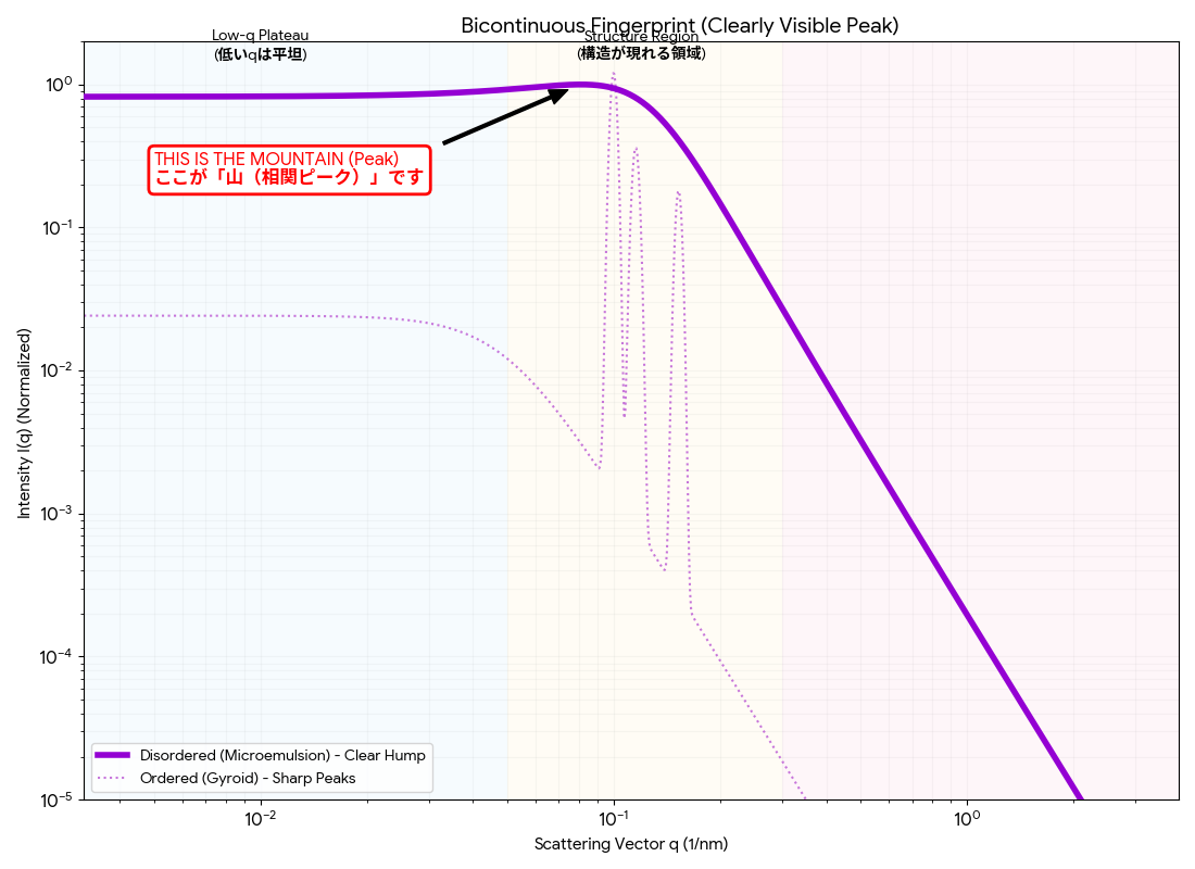
No. 09 Disordered Bicontinuous
A structure seen in the initial phase separation of microemulsions or polymer blends. Two phases fill the space and intertwine, but without long-range regularity (crystal-like order).
1. 'Fingerprint' to look for
- Correlation Peak (Broad Hump): Focus on the thick purple solid line. The sharp multiple peaks seen in the ordered phase disappear, and a single broad hump appears. This indicates that while there is no strict periodicity, there is an 'average mesh size'.
- Low-angle Plateau: The intensity settles to a constant value or decreases slightly towards q → 0. This reflects the nature of the space being completely filled, causing scattering to cancel out at ultra-long distances.
- High-angle Porod Decay: Ultimately decays along q−4.
2. Main Analytical Indicators
Identify the 'average mesh size' (domain spacing D) of the fluctuating maze.
- Calculation of Mesh Size: Derived from the peak position q*:
D (Average domain spacing) ≈ 2π / q*
Example: If the peak is at q = 0.1 nm−1, the mesh size of the maze is approximately 63 nm.
3. Crucial differences from the Ordered Phase (No. 10)
- Ordered Phase: Multiple sharp, spiky peaks.
- Disordered Phase: A single blurred hump.
NanoTerasu Application Advice
Capturing the moment the 'spikes turn into a hump' by changing experimental conditions (temperature or concentration) is definitive proof of a phase transition from a crystalline maze to a fluid maze. Precise determination of the broad peak position in the disordered phase requires smooth data with low noise.
Note: If this broad hump sits on top of a steeply decaying background, it may appear merely as a subtle 'shoulder' or become completely obscured. Performing proper background subtraction or utilizing emphasized plots with the vertical axis converted to I(q) · q2 or I(q) · q4 (keeping the horizontal axis as q) is often necessary to clearly reveal the peak position.
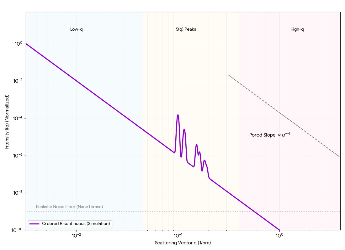
No. 10 Ordered Bicontinuous
A 'periodic maze' structure that fills the entire space, observed in materials such as the gyroid phase of block copolymers, cubic liquid crystals formed by lipids (cubosomes), and mesoporous silica (e.g., MCM-48). At synchrotron facilities like NanoTerasu, beautiful decay curves spanning over 10 orders of magnitude dynamic range, as seen in this graph, can be captured.
1. Reading the Graph
- Low-q (Global): Reflects the overall spatial arrangement of the structure.
- Structured Peak: Sharp peaks indicating the regularity (periodicity) of the maze.
- High-q Porod Region: By extending the y-axis, the q−4 decay reflecting the sharpness of the interface can be seen clearly over several orders of magnitude.
2. Main Analytical Indicators
Identify the 'period' (domain spacing D) of the periodic maze.
- Calculation of Period D: Derived from the position of the fundamental peak q*:
D ≈ 2π / q*
Example: If q* = 0.1 nm−1, the period D is approximately 63 nm.